Should You Buy or Rent? The Honest Math
Why this exists
You often hear: buy a house, because rent is throwing money away. That framing ignores opportunity cost: the money you put into the down payment, mortgage principal payments, property tax, insurance, and maintenance could have been invested in other assets, like the stock market. Considering all the factors and their impact on this decision is non-trivial.
For context, here’s how the two have actually behaved over the past 20 years:
I built a thoughtful simulation using system2 to answer this question with sound math and clear explanations. It’s tailored for the US, with dropdowns for your state (50 + DC), filing status, and federal bracket, all driving the tax calculations. Nine sliders let you dial in the financial details: home price, rent, mortgage rate, down payment, returns, time horizon, and more.
Hover the ⓘ icon next to any field to see what it means. The methodology section below walks through every assumption, simplification, and equation.
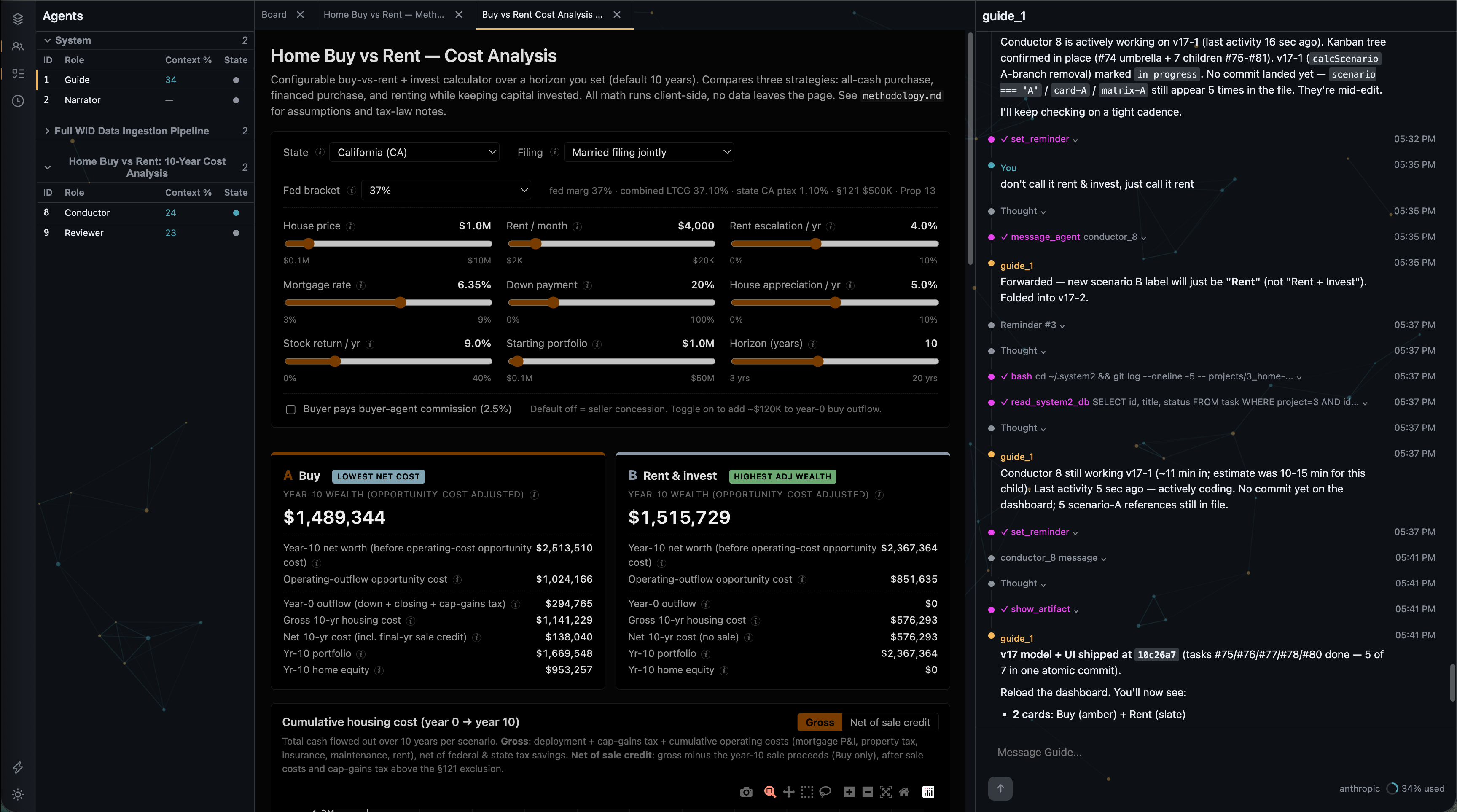
Here’s a snapshot of system2 in action while building this:
The model
Methodology
Companion document to the dashboard. Defines every input, the math, the tax-law specifics, the design choices, and every documented simplification.
What it models. Two housing strategies over a user-chosen horizon, for any U.S. tax jurisdiction:
- A — Buy: purchase a home with a configurable down payment (0% – 100%). At 0–99% down, the rest is financed with a 30-year fixed jumbo mortgage. At 100% down, the purchase is all-cash with no loan. Sell at year N.
- B — Rent: keep the portfolio untouched; pay rent that escalates annually.
The headline metric is opportunity-cost-adjusted year-N wealth: base net worth minus the future value of annual housing outflows that could otherwise have stayed invested. The cash-cost view (gross / net N-year housing cost) is kept alongside for the cash-budgeting question.
Parameterized inputs. House price, rent, rent escalation, mortgage rate, down payment, house appreciation, stock return, starting portfolio, and horizon are sliders. US state (50 states + DC), filing status (MFJ / Single / HoH), and federal marginal bracket (22 / 24 / 32 / 35 / 37%) are dropdowns. Buyer-agent commission is an advanced-options checkbox.
The math is fully parameterized by the inputs above. This document together with the live dashboard describes everything the model does; concrete numbers for any input combination come from running the dashboard.
How to read the dashboard (5-minute orientation)
The dashboard answers two coordinated questions:
- “How much money is needed?” — total housing-related cash that flows out of your pocket over the selected horizon, per scenario. Captured by the Cumulative housing cost chart and the Gross N-yr housing cost / Net N-yr cost rows on the summary cards.
- “What’s the honest wealth comparison?” — year-N net worth after subtracting the future value of annual housing outflows that could otherwise have remained invested. Captured by the Opportunity-cost-adjusted wealth lead number on each summary card, the adjusted wealth trajectory chart, and the sensitivity matrix. Year-N net worth (before operating-cost opportunity cost) is also shown as a secondary row for transparency.
The two views aren’t redundant. View 1 isolates housing cash cost; View 2 converts those cash costs into their year-N opportunity cost at the stock-return slider rate. View 2 is the headline because treating annual housing costs as if they were funded externally (and therefore charged nothing in opportunity cost) is useful for cash budgeting but too favorable to high-operating-cost scenarios as a wealth comparison.
The 9 sliders (house price, rent, rent escalation, mortgage rate, down payment, house appreciation, stock return, starting portfolio, horizon) control the live state. The 3×3 sensitivity matrix uses fixed grid axes (stock 6/9/12% × appreciation 3/5/7%) regardless of slider state — a black box on each small-multiple shows the cell nearest to your current slider position.
Every labeled input and summary card field has a small ⓘ info button to its right. Hover (desktop) or click (touch / keyboard-accessible) to see a description of what that field means and how it’s computed. This is layered on top of the methodology — the info buttons are quick-reference, this document is the authoritative explanation.
Scenarios
| A — Buy | B — Rent | |
|---|---|---|
| Year-0 cash deployed for purchase | $$\text{down} \times \text{price}$$ + closing (+ optional buyer commission) | $0 |
| Mortgage | 30-year fixed at slider rate, on $$(1 - \text{down}) \times \text{price}$$. None at $$\text{down} = 100\%$$. | n/a |
| Operating costs | mortgage P&I (zero at $$\text{down} = 100\%$$) + property tax + insurance + maintenance | rent (no other costs) |
| Tax savings | federal mortgage interest (up to $750K cap; zero at $$\text{down} = 100\%$$) + state mortgage interest (up to state cap; zero at $$\text{down} = 100\%$$) + property tax (federal SALT-capped + state) | none |
| Year-N event | sell house, realize equity, pay off remaining loan (none at $$\text{down} = 100\%$$) | nothing |
Note: all-cash purchase. An all-cash purchase is modeled by setting the down-payment slider to 100% in Scenario A. At that slider value the loan amount is zero, no mortgage interest is paid, no federal or state mortgage-interest deduction is taken, and the year-0 deployment equals the full price plus closing (plus optional buyer commission). The same Scenario A code path handles both financed and all-cash purchases; down-payment percentage is the only difference.
Modeling decisions
| Topic | Decision | Rationale |
|---|---|---|
| Combined LTCG rate | Federal LT bracket + 3.8% NIIT + state LTCG component. | Federal LT rate derives from the federal-marginal dropdown (15% at marginal ≤ 35%, 20% at 37%; documented simplification). NIIT is always-on. State LTCG defaults to state ordinary marginal rate, with documented exceptions for HI, MA, and WA (see State tax data sources). For an MFJ household at the default 32% federal marginal in California: 15% + 3.8% + 13.3% = 32.1%. |
| Mortgage interest deduction caps | Federal and state caps modeled as separate layers. | Federal cap is $750K of principal (TCJA). State caps default to $750K (federal conformity); the canonical exception is California, which under Cal. R&T §17072 still allows the pre-TCJA $1M cap. See Mortgage-interest deduction caps in the Math section for the layered formula. |
| No PMI | Warning banner shown when down-payment slider < 20%. | Jumbos typically don’t carry PMI — lenders use piggyback (80/10/10) or require 10–20%+ down. Modeling PMI for a configuration that wouldn’t be financed that way would be misleading. |
| Two wealth metrics | Base ledger compounds the portfolio untouched after year 0; the headline decision metric subtracts the future value of annual operating outflows. | The cash-cost view answers “how much money is needed?” The wealth-decision view recognizes that annual housing costs still displace investable cash. Both are surfaced: gross / net N-yr cost rows for cash, opportunity-cost-adjusted wealth for the wealth comparison. |
| Stock cost basis ≈ 0 | 100% taxable gain on the stock liquidated for year-0 deployment. | Modeling assumption — set consciously. If the basis on the stock you would actually sell is materially non-zero, the year-0 cap-gains tax is overstated proportionally and Scenario A (Buy) looks better than the dashboard shows. |
| Symmetric year-0 cap-gains drag | Year-0 cap-gains tax applies uniformly to whatever stock each scenario liquidates. | Same source of capital, same tax law: the differential is purely a function of how much stock each scenario liquidates. Year-0 outflow rows on the dashboard show the dollar values for the current slider state. |
| Sensitivity matrix layout | 2 small-multiples (Buy + Rent) + 1 binary winner-region matrix (Buy vs Rent). | Most information-dense option. Each per-scenario matrix uses a warm-shades single-hue palette (darker = higher value, per-scenario scale); the winner-region matrix reads at a glance. |
| Slider-point overlay | Black outline on the nearest grid cell of each small-multiple. | Off-grid slider state (e.g. stock = 11%, apprec = 4%) snaps to nearest. Approximates a continuous-coord overlay. |
| Buyer-agent commission | Advanced-options checkbox. Default off (seller concession). | Toggle adds 2.5% × purchase to the Buy scenario’s year-0 outflow. Post-2024 NAR settlement made buyer-side commission a separately-negotiated item. |
| State picker | Drives state ordinary marginal rate, state LTCG component, state standard deduction, state mortgage-interest cap, effective property tax rate, and property-tax growth regime. | Two growth regimes: prop13 (California, 2%/yr assessed-value cap) and market (all other states, base reassessed annually with market value). See State tax data sources below for per-state values, the HI / MA / WA LTCG exceptions, and the Texas / Florida property-tax shelters not modeled. |
| Filing-status dropdown | MFJ / Single / HoH drives the federal standard deduction and the §121 home-sale exclusion. | Federal standard deductions for 2026: MFJ $30,800, Single $15,750, HoH $23,625. §121 exclusion: MFJ $500K, Single $250K, HoH $250K (IRS §121(b) treats HoH like Single). Affects both the itemized-vs-standard comparison and the year-N cap-gains tax on the home sale. |
| Federal-marginal dropdown | 22% / 24% / 32% / 35% / 37%. Drives the federal-side itemized-deduction value AND the federal LTCG rate via the simplified mapping 15% for marginal ≤ 35%, 20% for 37%. | Documented simplification: real federal LTCG depends on taxable-income thresholds ($94K MFJ 0% / $583K MFJ 15% / above 20%), not directly on marginal bracket. For top-bracket users the mapping is exact; for users in the 22-35% brackets it assumes top-of-bracket income, so 15% is the floor (not 0%). NIIT 3.8% modeled as always-on. |
Year-0 cap-gains tax treatment
Both the deployment AND the year-0 cap-gains tax bill leave the portfolio at year 0. The cap-gains tax is computed first-order on the realized gain (no infinite gross-up cascade). At the default sliders (CA / MFJ / 32% federal marginal, $1,000,000 house, $1,000,000 starting portfolio, down = 20%), Scenario A (Buy) resolves as:
deployment      = 0.20 × $1,000,000 + 1.5% × $1,000,000 = $215,000
cg_tax_y0       = $215,000 × 32.1%                      = $69,015    [combined LTCG: 15% fed + 3.8% NIIT + 13.3% CA]
year-0 outflow  = $215,000 + $69,015                    = $284,015
portfolio_y0    = $1,000,000 − $284,015                  = $715,985
At down = 100% (all-cash), the formula gives:
deployment      = 1.00 × $1,000,000 + 1.5% × $1,000,000 = $1,015,000
cg_tax_y0       = $1,015,000 × 32.1%                    = $325,815   [combined LTCG: 15% fed + 3.8% NIIT + 13.3% CA]
year-0 outflow  = $1,015,000 + $325,815                 = $1,340,815
portfolio_y0    = $1,000,000 − $1,340,815               = −$340,815
Year-0 outflow ($1,340,815) exceeds the $1M starting portfolio — the low-capital coverage warning fires.
The cap-gains tax is real cash leaving total wealth; it appears as part of year-0 housing cost AND is deducted from the portfolio at year 0. No infinite gross-up cascade because in practice an April tax bill is funded from many sources (quarterly estimates, dividends, short-term cash) without triggering a recursive sequence of stock sales. First-order is the honest approximation at this granularity.
Tax-constant detail
Three tax constants have nuances worth spelling out before the math:
Combined LTCG rate
\[ \begin{align*} \text{ltcg\_combined} &= \text{federal\_LT\_rate} + 3.8\% \text{ NIIT} + \text{state\_LTCG} \\ \text{federal\_LT\_rate} &= \begin{cases} 20\% & \text{if } \text{federal\_marginal} \geq 37\% \\ 15\% & \text{otherwise} \end{cases} \end{align*} \]The federal LT rate is mapped from the marginal-bracket dropdown via a simplification — the real bracket boundary is taxable-income-based, not marginal-bracket-based. NIIT is always-on. The state LTCG component defaults to state ordinary marginal rate (the state lookup overrides this for HI / MA / WA — see below).
California breakdown at the top federal bracket: 20% federal LT + 3.8% NIIT + 13.3% CA = 37.1%. CA’s 13.3% top rate already embeds the 1% Mental Health Services Tax surcharge (12.3% statutory top + 1% MHST per Prop 63 / Cal. R&T §17043 = 13.3% all-in); naively adding “+ 1% MHST” on top would double-count and give 38.2%.
HI / MA / WA exceptions: see the State tax data sources table — Hawaii caps LT capital gains at 7.25%, Massachusetts uses a flat 5% on LT gains, and Washington imposes a 7% tax on capital-gains income only (no general state income tax).
SALT cap
The 2026 headline federal SALT cap is $40,400 (Working Families Tax Cut Act 2025 raised TCJA’s $10K and indexed +1%/yr through 2029, reverting to $10K in 2030). The cap phases down at 30% of MAGI excess above $505K MAGI, floored at $10K. At top-bracket federal income (37% bracket → MAGI ≥ $731K MFJ), MAGI sits far above the phase-down threshold so the cap fully phases down to its $10K floor.
Net effect: the model treats federal SALT as a constant $10K contribution to itemized deductions (the phase-down floor), independent of state and property tax. This matches reality whenever actual state income tax + property tax ≥ $10K — satisfied at canonical anchor prices in both high-state-income-tax states (state income tax fills the cap at top federal income) and no-state-income-tax states (property tax fills it at typical house prices). See Simplifications #16 for the narrow edge case where this slightly overstates Buy’s federal tax savings.
No U.S. state imposes a federal-style SALT cap on its own income tax return, so the state-side property-tax deduction is $$\text{property\_tax} \times \text{state\_marginal}$$ with no cap.
State mortgage-interest deduction conformity
Most states conform to the federal $750K TCJA cap by default. The canonical exception is California, which under Cal. R&T §17072 still allows the pre-TCJA $1M cap. The model applies federal and state caps as separate deduction layers; see the math section below for the formula.
State tax data sources
State-level constants used by the model are drawn from consolidated 2025 reference tables; per-state primary-source citation (state revenue department schedules) is out of scope for this analytical tool but recommended for any tax-prep-grade use.
| Field | Source |
|---|---|
| Top marginal income rate (MFJ) | Tax Foundation, “2025 State Individual Income Tax Rates and Brackets” (taxfoundation.org/data/all/state/state-income-tax-rates/), top bracket per state as of January 1, 2025. |
| MFJ standard deduction | Same source. For states without a standard deduction (CT, IL, IN, MA, MI, NJ, OH, WV), the MFJ personal exemption (Couple column) is used as the proxy so the itemized-vs-standard comparison still functions. States with neither standard deduction nor personal exemption (PA, FL, TX, NV, SD, TN, WY, NH, AK, WA, UT, IA) are set to 0 (state-side mortgage interest deduction collapses to itemized × marginal). |
| State LTCG component | Defaults to state ordinary marginal rate (most states tax LT capital gains as ordinary income). Documented exceptions: Hawaii — alternative capital-gains tax caps LT gains at 7.25% (HRS §235-51) below the 11% top marginal; Massachusetts — flat 5% on LT capital gains regardless of the 9% top marginal on >$1M income; Washington — 7% capital-gains-only tax above the $270K MFJ threshold, with no general state income tax. |
| Mortgage interest deduction cap | Federal $750K (TCJA) assumed for all states except California, which under Cal. R&T §17072 still allows the pre-TCJA $1M cap. Other states with possible non-conformity (AR, MS) are modeled at $750K as a conservative simplification. |
| Property tax effective rate | U.S. Census Bureau ACS 2024 aggregates (B25090 / B25082) for owner-occupied housing, consolidated in the Tax Foundation “Property Taxes by State 2026” series. California exception: the model uses 1.1% (representative of high-burden CA county jurisdictions, where local school and special-district levies push effective rates above the state-wide average) rather than the 0.69% ACS state-wide figure. |
| DC property tax | Tax Foundation 2025 estimate (~0.55% effective). ACS aggregates only cover 50 states. |
| Property tax growth regime | prop13 (California only): assessed value capped at +2%/yr regardless of market. market (all other states): base reassessed annually with the house-appreciation slider rate. Texas homestead caps, Florida Save Our Homes, Michigan PRE, and similar protections are NOT modeled — flagged simplification. |
Known state-level simplifications
- Top marginal bracket only. No income-level differentiation across state brackets. Itemized-deduction value computed at top state marginal.
- State-wide effective property tax rate. Real rates vary materially by county and municipality — see Tax Foundation’s county-level data for finer resolution.
- No state-level SALT cap on its own return. No U.S. state imposes a federal-style SALT cap on its own income tax return; the model uses 0 as the state-side SALT cap by default.
- Locality income taxes not modeled (NYC, Philadelphia, Maryland counties, etc.). These add 1-4% to the effective state rate in affected jurisdictions.
- Filing status and federal marginal bracket are exposed as dropdown inputs (MFJ/Single/HoH; 22/24/32/35/37% common bracket points). Federal LTCG rate derives from marginal bracket via the simplified mapping (15% for marginal ≤ 35%, 20% for 37%); actual federal LTCG depends on taxable-income thresholds not modeled here. NIIT 3.8% modeled as always-on regardless of MAGI threshold.
- Washington real-estate exclusion is modeled. WA’s 7% capital gains tax (RCW 82.87) explicitly excludes real estate (RCW 82.87.050(8)). State-side LTCG on year-0 stock liquidation correctly applies the 7% rate; state-side LTCG on year-N home sale correctly applies 0%. Federal LT + NIIT still apply to both.
- Massachusetts Millionaire’s Surtax (4% on income > $1M, Massachusetts Constitution Article XLIV §2, effective 2023) is not modeled. The model uses a flat 5% state LTCG for MA. For top-income MA users, the surtax applies to capital gains above the $1M MAGI threshold, so state LTCG should be 5% on the portion below and 9% above. At a $4.799M home sale with $500K §121 exclusion, this understates state tax by roughly $80K (≈4% × the gain amount in surtax range).
Inputs
Fixed parameters
Universal constants used regardless of state / filing / federal bracket. (Per-state values for marginal, LTCG, std deduction, mortgage cap, property tax rate, and growth regime are in the State tax data sources table. Per-filing federal standard deductions and §121 exclusion are in the Categorical inputs table below.)
| Constant | Value | Notes |
|---|---|---|
| NIIT | 3.8% | Federal surtax on net investment income > $250K MFJ MAGI threshold. Modeled as always-on (Simplification #2). |
| Federal mortgage interest cap | $750,000 of principal | TCJA (assumed conformance for all states except CA per the State tax data sources table). |
| Property tax growth — Prop 13 regime | 2%/yr | California only. State.ptaxRegime === ‘prop13’. |
| Property tax growth — market regime | tracks house-appreciation slider | All non-CA states. State.ptaxRegime === ‘market’. |
| Insurance | 0.35% × market value/yr | Typical non-catastrophe-zone premium. |
| Maintenance | 0.4% yrs 1-5, 0.8% yrs 6-10, 1.2% yrs 11-15, 1.6% yrs 16-20 | New-construction warranty period, settled-house period, mid-life systems, major-systems replacement era. Long-run average ~1%/yr matches industry rule of thumb. Schedule extends to year 20 to support the horizon slider. |
| Closing costs | 1.5% × price | Industry typical (escrow, title, transfer tax, inspections). |
| Sale costs | 6% × sale price | 5% commissions + 1% title/transfer. Conservative — 2025 post-NAR-settlement averages are ~5%, possibly as low as 3-3.5% if the seller only pays own agent. Held at 6% to reflect high-cost-coastal luxury-segment stickiness. |
| Buyer-agent commission (toggle on) | 2.5% × price | Post-2024 NAR settlement; default off. |
| Stock cost basis fraction | 0 (100% gain) | Modeling assumption — sets year-0 stock liquidation as fully LTCG-taxable. |
| Loan term | 30 years (360 months) | Standard fixed-rate jumbo. |
Categorical inputs (dropdowns)
| Input | Options | Default |
|---|---|---|
| US state | 50 states + DC | California |
| Filing status | MFJ / Single / HoH | MFJ |
| Federal marginal bracket | 22% / 24% / 32% / 35% / 37% | 32% |
Per-filing-status federal constants:
| Status | Federal std deduction (2026) | §121 exclusion |
|---|---|---|
| MFJ | $30,800 | $500,000 |
| Single | $15,750 | $250,000 |
| HoH | $23,625 | $250,000 (IRS §121(b) treats HoH as Single) |
Per-bracket federal LTCG (simplified mapping):
| Federal marginal | Federal LT rate |
|---|---|
| 22 / 24 / 32 / 35% | 15% |
| 37% | 20% |
Sliders (live)
| Slider | Range | Step | Default |
|---|---|---|---|
| House price | $100,000 – $10,000,000 | $1,000 | $1,000,000 |
| Rent / month | $1K – $20K | $500 | $4,000 |
| Rent escalation / yr | 0% – 10% | 0.5% | 4% |
| Mortgage rate / yr | 3% – 9% | 0.05% | 6.35% |
| Down payment | 0% – 100% | 5% | 20% |
| House appreciation / yr | 0% – 10% | 0.5% | 5% |
| Stock return / yr | 0% – 40% | 0.5% | 9% |
| Starting portfolio | $100,000 – $50,000,000 | $100,000 | $1,000,000 |
| Horizon | 3 – 20 years | 1 year | 10 years |
Math
Mortgage amortization
Standard US convention: monthly amortization on the financed amount.
\[ \begin{align*} \text{loan} &= \text{price} \times (1 - \text{down}) \\ r_m &= \text{mortgage\_rate} / 12 \\ \text{payment}_m &= \text{loan} \times \frac{r_m (1 + r_m)^{360}}{(1 + r_m)^{360} - 1} \end{align*} \]For each month $$m$$:
\[ \begin{align*} \text{interest}_m &= \text{balance}_{m-1} \times r_m \\ \text{principal}_m &= \text{payment}_m - \text{interest}_m \\ \text{balance}_m &= \text{balance}_{m-1} - \text{principal}_m \end{align*} \]For each year $$t$$ (months $$12(t-1)+1$$ through $$12t$$), aggregate the monthly results into a year-$$t$$ record. The dot is field-access notation (struct-style): $$\text{year}_t\mathord{.}\text{interestPaid}$$ reads “the interestPaid field of the year-$$t$$ record,” matching the dashboard’s years[t-1].interestPaid shape.
Tax savings from buying vs renting (federal + state, with standard-deduction baseline)
The federal tax saved by buying equals $$(\text{itemized\_buy} - \text{fed\_standard}) \times \text{federal\_marginal}$$, not $$\text{gross\_deductible\_interest} \times \text{federal\_marginal}$$. The rent baseline is fed_standard because rent’s only itemized item (SALT) is below the federal standard deduction. The same logic applies on the state return with the state standard deduction (or the personal-exemption proxy for states without a standard deduction; see State tax data sources).
Mortgage-interest deduction caps (principal-side)
\[ \begin{align*} \text{fed\_ded\_frac}_t &= \frac{\min(\text{fed\_cap},\, \text{year}_t\mathord{.}\text{avgBalance})}{\text{year}_t\mathord{.}\text{avgBalance}} \\ \text{state\_ded\_frac}_t &= \frac{\min(\text{state\_cap},\, \text{year}_t\mathord{.}\text{avgBalance})}{\text{year}_t\mathord{.}\text{avgBalance}} \\ \text{fed\_ded\_int}_t &= \text{year}_t\mathord{.}\text{interestPaid} \times \text{fed\_ded\_frac}_t \\ \text{state\_ded\_int}_t &= \text{year}_t\mathord{.}\text{interestPaid} \times \text{state\_ded\_frac}_t \end{align*} \]Federal: itemized = mortgage interest + SALT floor ($10K); compared to the federal standard deduction.
\[ \begin{align*} \text{fed\_itemized}_t &= \text{fed\_ded\_int}_t + \$10{,}000 \\ \text{fed\_savings}_t &= \max(0,\ \text{fed\_itemized}_t - \text{fed\_std}) \times \text{federal\_marginal} \end{align*} \]State: itemized = mortgage interest + property tax (no state-side SALT cap on own return).
\[ \begin{align*} \text{state\_itemized}_t &= \text{state\_ded\_int}_t + \text{property\_tax}_t \\ \text{state\_savings}_t &= \max(0,\ \text{state\_itemized}_t - \text{state\_std}) \times \text{state\_marginal} \end{align*} \]Where fed_cap, state_cap are the mortgage-interest caps; fed_std is per filing status (Categorical inputs); state_std and state_marginal come from the state picker.
Both federal and state caps bind every year whenever the average loan balance stays above the higher cap. Example: a $3.84M loan at 6.35% over 10 years keeps the average balance above $1M throughout, so under CA’s $1M cap, ded_frac averages ≈ 26% on the state side and ≈ 20% on the federal side ($750K cap). When the loan amortizes below the federal cap, the federal ded_frac rises toward 1.
Property-tax deduction
In the model, property tax does not flow into the federal itemized total — the federal SALT contribution is captured as a constant $10K addition to federal itemized deductions (see Simplifications #16), independent of state and property tax. On the state return, property tax does flow into the state itemized total above; equivalently:
\[ \text{property\_tax}_t = \text{price} \times \text{state.ptaxRate} \times (1 + \text{ptax\_growth})^{t-1} \]where
\[ \text{ptax\_growth} = \begin{cases} 0.02 & \text{if state.ptaxRegime} = \text{`prop13' (California)} \\ \text{house\_appreciation} & \text{otherwise (market reassessment)} \end{cases} \]\[ \text{state\_ptax\_savings}_t = \text{property\_tax}_t \times \text{state\_marginal} \qquad [\text{when state itemizes; embedded in state\_savings}_t \text{ above}] \]Insurance and maintenance
Both scaled to current market value (simplification: real insurance is replacement-cost-based; real maintenance is bumpy year-to-year).
\[ \begin{align*} \text{market\_value}_t &= \text{price} \times (1 + \text{house\_appreciation})^t \\ \text{insurance}_t &= \text{market\_value}_t \times 0.35\% \\ \text{maint}_t &= \text{market\_value}_t \times \text{maint\_rate}_t \\ &\qquad [0.4\% \text{ yrs } 1\text{--}5,\ 0.8\% \text{ yrs } 6\text{--}10,\ 1.2\% \text{ yrs } 11\text{--}15,\ 1.6\% \text{ yrs } 16\text{--}20] \end{align*} \]Per-scenario annual cash outlay (years 1..N)
For Scenario A (Buy), state_savings_t is the result of the Tax savings calc above (which already folds in state mortgage interest + state property tax inside the itemized total). fed_savings_t similarly folds in federal mortgage interest + the SALT-capped property tax deduction.
Scenario A — Buy:
\[ \begin{align*} \text{gross\_A}_t &= 12 \times \text{payment}_m + \text{property\_tax}_t + \text{insurance}_t + \text{maintenance}_t \\ \text{savings\_A}_t &= \text{fed\_savings}_t + \text{state\_savings}_t \\ \text{net\_A}_t &= \text{gross\_A}_t - \text{savings\_A}_t \end{align*} \]At $$\text{down} = 100\%$$ the loan amount is zero, so $$\text{payment}_m = 0$$, $$\text{interest\_paid}_t = 0$$, the mortgage-interest deduction component is zero, and the itemized total collapses to property tax. Both the federal and state savings then equal $$\max(0,\ \text{property\_tax} + \text{SALT} - \text{std}) \times$$ the respective marginal rate. The formula above subsumes the all-cash case naturally — no separate branch.
Scenario B — Rent:
\[ \begin{align*} \text{monthly\_rent}_t &= \text{rent} \times (1 + \text{rent\_esc})^{t-1} \qquad [\text{annual reset on renewal}] \\ \text{net\_B}_t &= 12 \times \text{monthly\_rent}_t \qquad [\text{no tax savings on rent}] \end{align*} \]Year-0 deployment and cap-gains tax
\[ \begin{align*} \text{buyer\_commission} &= \begin{cases} 2.5\% \times \text{price} & \text{if checkbox on} \\ 0 & \text{otherwise} \end{cases} \\ \text{closing} &= 1.5\% \times \text{price} \end{align*} \]Scenario A (Buy) scales linearly with down payment. At $$\text{down} = 100\%$$ it collapses to full price + closing (+ commission) — the all-cash case. At $$\text{down} = 0\%$$ it is just closing + commission — full-loan jumbo (with the standard warning).
\[ \begin{align*} \text{deployment\_A}_{y0} &= \text{down} \times \text{price} + \text{closing} + \text{buyer\_commission} \\ \text{deployment\_B}_{y0} &= 0 \qquad [\text{Rent: no deployment}] \end{align*} \]100% gain assumption: tax = deployment × combined LTCG, paid from portfolio.
\[ \begin{align*} \text{cg\_tax\_A}_{y0} &= \text{deployment\_A}_{y0} \times \text{ltcg\_combined} \\ \text{cg\_tax\_B}_{y0} &= 0 \\ \text{year0\_cost}_X &= \text{deployment\_X}_{y0} + \text{cg\_tax\_X}_{y0} \\ \text{portfolio\_y0}_X &= \text{capital} - \text{deployment\_X}_{y0} - \text{cg\_tax\_X}_{y0} \end{align*} \]Portfolio compounding (years 1..N)
Annual compounding, end-of-year convention. In the base ledger, portfolio is untouched by operating costs after year 0; the adjusted-wealth metric separately subtracts the future value of those annual outflows as an opportunity-cost adjustment.
\[ \text{portfolio}_t = \text{portfolio}_{t-1} \times (1 + \text{stock\_return}) \]Year-N sale (Buy only)
Per IRS §1001(b), “amount realized” on a sale equals sale price minus selling expenses. Selling expenses (commissions, title, transfer tax) reduce the gain before the §121 exclusion, not just the cash proceeds.
\[ \begin{align*} \text{market\_value}_{yN} &= \text{price} \times (1 + \text{house\_appreciation})^N \\ \text{gross\_proceeds} &= \text{market\_value}_{yN} \times (1 - 6\%) \qquad [\text{sale costs: 5\% commissions + 1\% title/transfer}] \\ \text{amount\_realized} &= \text{gross\_proceeds} \qquad [\S 1001(b)\text{: net of selling expenses}] \\ \text{gain} &= \text{amount\_realized} - \text{price} \qquad [\text{purchase price} = \text{basis; improvements ignored}] \\ \text{taxable\_gain} &= \max(0,\ \text{gain} - \text{sec121\_exclusion}) \\ &\qquad [\text{sec121\_exclusion: }\$500\text{K MFJ} / \$250\text{K Single} / \$250\text{K HoH}] \\ \text{cg\_tax\_sale} &= \text{taxable\_gain} \times \text{ltcg\_combined\_re} \\ &\qquad [\text{year-}N\text{ rate; differs from year-0 only in WA per Simp.\ \#6}] \\ \text{remaining\_loan} &= \text{balance after month } 12N \quad (0 \text{ at } \text{down} = 100\%) \\ \text{net\_from\_sale} &= \text{gross\_proceeds} - \text{cg\_tax\_sale} - \text{remaining\_loan} \end{align*} \]where $$\text{ltcg\_combined\_re} = \text{fed\_LTCG} + \text{NIIT} + \text{state.ltcg\_re}$$, with $$\text{state.ltcg\_re} = 0$$ for Washington (RCW 82.87.050(8) excludes real estate from the state capital gains tax) and $$\text{state.ltcg\_re} = \text{state.ltcg}$$ for all other states. The distinction matters only in WA — every other state uses the same combined LTCG rate for year-0 stock liquidation and year-N home sale.
Cumulative cost views (the “how much money is needed” headline)
\[ \begin{align*} \text{cum\_gross}_X &= \text{year0\_cost}_X + \sum_{t=1}^{N} \text{gross}_{X,t} \\ \text{cum\_net}_X &= \text{year0\_cost}_X + \sum_{t=1}^{N} \text{net}_{X,t} - \text{net\_from\_sale}_X \end{align*} \]The first omits tax savings and sale credit. The second is tax-savings-adjusted and nets the sale credit ($$\text{net\_from\_sale}_B = 0$$ for Rent).
Both are surfaced on the summary cards. Toggle on the cumulative-cost chart switches between them.
Year-N net worth (base ledger)
\[ \text{net\_worth}_{X,\, yN} = \text{portfolio}_{X,\, yN} + \begin{cases} \text{net\_from\_sale}_A & \text{for Buy} \\ 0 & \text{for Rent} \end{cases} \]The base-ledger net worth appears on each summary card as a secondary row labeled “Year-N net worth (before operating-cost opportunity cost).” It captures year-0 deployment opportunity cost because the portfolio starts lower by the year-0 outflow, but it does not charge annual housing outflows for the investment returns those dollars could have earned.
Opportunity-cost-adjusted wealth (headline metric)
The wealth comparison that handles annual outflows honestly asks: if each annual housing outflow had not been spent on housing, what would it be worth at the stock-return slider rate by year N?
\[ \begin{align*} \text{opp\_cost}_{X,\, yN} &= \sum_{t=1}^{N} \text{net}_{X,t} \times (1 + \text{stock\_return})^{N-t} \\ \text{adjusted\_wealth}_{X,\, yN} &= \text{net\_worth}_{X,\, yN} - \text{opp\_cost}_{X,\, yN} \end{align*} \]Where $$\text{net}_{X,t}$$ is the existing year-by-year tax-savings-adjusted outflow:
- A (Buy): mortgage P&I (zero at $$\text{down} = 100\%$$) + property tax + insurance + maintenance − tax savings
- B (Rent): rent (no tax savings)
Year-0 outflow is not included in $$\text{opp\_cost}_{X,\, yN}$$, because the base ledger already subtracts it from the starting portfolio ($$\text{capital} - \text{y0\_outflow}$$) before compounding. Subtracting it again would double-count the same lost compounding.
The adjustment matters because the base-ledger net-worth metric implicitly treats ongoing housing costs as if they were paid from a source that had no alternative investment return. The adjusted metric treats every dollar spent on housing as a dollar that could otherwise have remained invested — the more rigorous wealth-decision metric. The gross/net cost rows remain the right answer to “how much cash is required?”
Price sensitivity of the Buy-vs-Rent winner
At low purchase prices, Scenario A (Buy) tends to beat Scenario B (Rent) on adjusted wealth because Buy’s operating outflows (mortgage P&I, property tax, insurance, maintenance) scale roughly proportionally with house price while Rent’s outflow stream is independent of price. As price rises, Buy’s outflow-stream future value at the stock-return slider rate outgrows the wealth gains from leveraged home appreciation, and Rent overtakes Buy.
The cross-over depends on every other slider — stock return, rent, rent escalation, mortgage rate, down payment, and house appreciation all shift the inflection. The dashboard’s price slider lets a user trace the cross-over for their own slider state; the sensitivity matrix small-multiples + binary winner-region heatmap visualize the broader landscape over the stock × appreciation grid.
Edge cases
| Slider state | Behavior |
|---|---|
| $$\text{down} = 100\%$$ | Scenario A is an all-cash purchase: no loan, no mortgage interest, no mortgage-interest deduction. Property tax still flows through the itemized-deduction calculation. Informational banner shows. |
| $$\text{down} = 0\%$$ | Full-loan jumbo. Warning banner: not realistic financing. Math still runs. |
| $$0 < \text{down} < 20\%$$ | Warning banner: jumbo lenders typically don’t offer this; PMI not modeled. |
| $$\text{house\_appreciation} = 0$$ | Scenario A pays 6% sale costs at year N with no offsetting gain → Buy is structurally favored only by tax shelter and equity build. Banner shows. |
| $$\text{stock\_return} = 0$$ | Portfolio doesn’t grow. Buy may dominate Rent even at modest appreciation. |
| Year-0 outflow exceeds starting portfolio | Warning banner names the slider levers to adjust (capital, price, or down payment). Math still produces finite output; the result is economically meaningless at that corner. |
Simplifications
Each simplification was a deliberate choice. Listed in rough order of impact.
- Operating costs are not modeled as literal portfolio drawdowns, but their opportunity cost is charged. The base ledger compounds the portfolio untouched after year 0 to avoid modeling taxable annual stock-liquidation mechanics; the adjusted-wealth metric then subtracts the future value of each tax-savings-adjusted annual outflow as if that cash could otherwise have remained invested. This is a wealth-comparison metric, not a cash-management forecast.
- AMT not modeled. The modeled deduction profile (SALT-capped at $10K floor, modest mortgage interest deduction due to TCJA cap) makes AMT very unlikely to bind at top-bracket income. AMT is dormant under TCJA at this income/deduction shape.
- NIIT modeled as always-on 3.8% on cap gains. For top-bracket users with investment income above the $250K MFJ MAGI threshold, NIIT applies fully; the model assumes that regime regardless of bracket selection.
- Federal vs CA AGI differences ignored. Symmetric itemized deductions assumed across federal and CA returns. Real differences are sub-percent.
- Marginal rates held constant 10 years. Bracket creep ignored. Inflation also not modeled — all values are nominal. To compare in real terms, mentally subtract an inflation rate from both
stock_returnandhouse_appreciationsliders. - Insurance scaled to market value. Real premiums are tied to replacement cost, which lags market value in a rising market and may exceed it in a falling one. Approximation acceptable at this granularity.
- Maintenance scaled to market value. Standard rule-of-thumb basis. Real-world spending is bumpy year-to-year.
- Property tax base. See Property-tax deduction in the Math section for the per-state formula.
ptax_growthis 2%/yr under California’s Prop 13 regime and the house-appreciation slider rate under market-reassessment regimes elsewhere. Per-state effective rates are the ACS state-wide averages; California is set to 1.1% to reflect high-burden CA county jurisdictions rather than the 0.69% state-wide average. Real county-level rates vary materially around the state-wide figure. - Cap-gains tax on year-0 sale = first-order. Tax on the gain from selling exactly
deploymentworth of stock. The gross-up cascade (where additional stock is sold to fund the tax, triggering more tax) is not modeled. In practice an April tax bill is funded from many sources (quarterly estimates, dividends, short-term cash) without triggering recursive stock sales, so first-order is the honest approximation. - Sale at exactly year 10 anniversary. Real sale timing is variable. §121 occupancy test (2-of-last-5-years) is trivially satisfied at 10 years.
- House sale basis = purchase price (no improvements; no closing-cost basis additions). New construction; improvement-basis additions are immaterial for a 10-year hold on a turn-key build. Per IRS Pub 530, capitalizable closing-cost additions to basis (title insurance, escrow fees, transfer/recording tax — typically ~50% of the 1.5% closing total, ~$36K) would lower the year-10 cap-gains tax bill by ~$13K — a sub-0.1% adjustment to year-10 net worth, omitted for simplicity. Mortgage points and prepaid items are not capitalizable.
- Buyer agent commission as a binary toggle. Real post-NAR-settlement market may settle at intermediate rates (1–3%); 0% or 2.5% is a coarse choice.
- Tax constants frozen at 2026 values. SALT cap reverts to $10K in 2030 (at top-bracket income the cap is already at the $10K floor due to phase-down, so this doesn’t matter). TCJA’s $750K mortgage interest cap also sunsets per current schedules — a future tax-law change would shift the deduction value materially. Forecasting tax-law changes is out of scope.
- Portfolio compounding annual, end-of-year. Stock-return slider is a nominal annual rate, applied as $$\times (1 + r)$$ at year-end. Monthly compounding ($$(1 + r/12)^{12} - 1$$) gives a slightly higher effective rate; difference is sub-percent at typical slider values.
- Rent escalation = annual reset on renewal. Within-year rent is flat; jumps $$\times (1 + \text{esc})$$ on the year boundary. Real lease behavior matches this.
- Federal SALT cap modeled as a uniform $10K contribution to itemized deductions across all states and federal-marginal-bracket selections. The 2026 headline cap is $40,400, phasing down at 30% of MAGI excess above $505K to a $10K floor; only at top-bracket federal income (37% → MAGI ≥ $731K MFJ) does the cap fully bottom out. The model uses the $10K floor uniformly across all federal-marginal-bracket selections because it does not separately track MAGI. The model also treats the SALT contribution to federal itemized as a constant $10K independent of the state-income-tax vs property-tax composition; this matches reality whenever the sum of actual state income tax + property tax is at least $10K (the cap binds in real law too). At canonical anchor prices that sum exceeds $10K in every modeled regime: high-state-income-tax states (CA, NY, MA, …) fill the cap from state income tax alone at top federal income, and no-state-income-tax states (AK, FL, NV, NH, SD, TN, TX, WA, WY) fill it from property tax alone at typical house prices (e.g., TX 1.245% × $4.8M = $59.7K ≫ $10K). The simplification slightly OVERSTATES Buy’s federal tax savings only in the narrow case of a no-state-income-tax state at a house price where property tax falls below $10K — at a $1M WA house (effective property-tax rate 0.737%, real property tax ≈ $7.4K), the overstatement is ~$973/yr fed savings at the 37% top bracket and
$4K cumulative cash overstatement over the 10-year horizon ($7K including opportunity-cost compounding at 9% stock return). Bounded above by $10K × fed_marginal per year. Falls to zero as house price scales up (at $2M WA, real property tax ≈ $14.7K ≥ $10K floor → model matches reality exactly).
Glossary
- LTCG: Long-term capital gains. Tax rate on gains from assets held > 1 year.
- NIIT: Net Investment Income Tax. 3.8% federal surtax on net investment income above $250K MFJ MAGI threshold.
- MHST: California Mental Health Services Tax (a.k.a. “millionaire’s tax”). 1% additional CA tax on income above $1M.
- SALT: State and Local Tax (income, sales, property). Federal deduction capped under TCJA / Working Families Tax Cut Act.
- §121: IRC §121 — primary residence capital gains exclusion ($500K MFJ, $250K single) on sale of a primary residence held / occupied 2 of the last 5 years.
- Prop 13: California Proposition 13 (1978) — caps assessed-value growth for property tax purposes at 2%/year regardless of market value, until sale.
- TCJA: Tax Cuts and Jobs Act (2017) — capped mortgage interest deduction at first $750K of principal for new loans, capped SALT at $10K, doubled standard deduction.
- PMI: Private Mortgage Insurance. Charged on conforming loans with < 20% down. Not standard for jumbo loans.
- MAGI: Modified Adjusted Gross Income. Used for many federal phase-outs, including SALT and NIIT.
- Jumbo loan: A mortgage above the conforming loan limit (~$766K in 2024 baseline, higher in high-cost counties). Does not qualify for purchase by Fannie Mae or Freddie Mac.
- Net cash from sale: Gross proceeds (sale price × 0.94) minus cap-gains tax (above §121 exclusion) minus remaining mortgage balance.